The resulting curve can be too jerky because of noise or imprecision. The coordinate values of the data can be smoothed by one of several approaches.
Smoothing with linear interpolation of adjacent values
Points in two-space can be smoothed by averaging adjacent points. In the simplest case, the two points, one on either side of an original point, P_i are averaged. Repeated applications of the linear interpolation to further smooth the data would continue to draw the reduced concave sections and faltten out the curve.
Smoothing with cubic interpolation of adjacent values
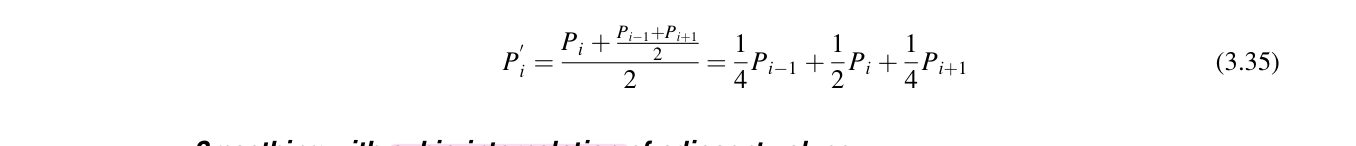
To preserve the curvature but still smooth the data, the adjacent points on either side of a data point can be used to fit cubic curve that is evaluated at its midpoint. This midpoints is averaged with the original point, as in the linear case. The two data points on either side of an original point, P_i, are used as constraints.

A cubic curve has the form shown in Equation 3.36. These equations can be used to solve for constants of the cubic curve (a, b, c, d). Equation 3.36 is evaluated at u=1/2; and the result is averaged wiwth the original data point.

For the end conditions, a parablic arc can be fit through the first, third, and fourth points, and an estimate for the second point from the start of the data set can be computed. The coefficient equation, P(u)=au^2+bu+c, can be computed and can be used to solve for the position P_1=P(1/3).

A similar procedure can be used to estimate the data point second from the end. The very first and very last data can be left alone if they represent hard constraints, or parabolic interpolation can be used to generate estimates for them as well.
Smoothing with convolution kernels
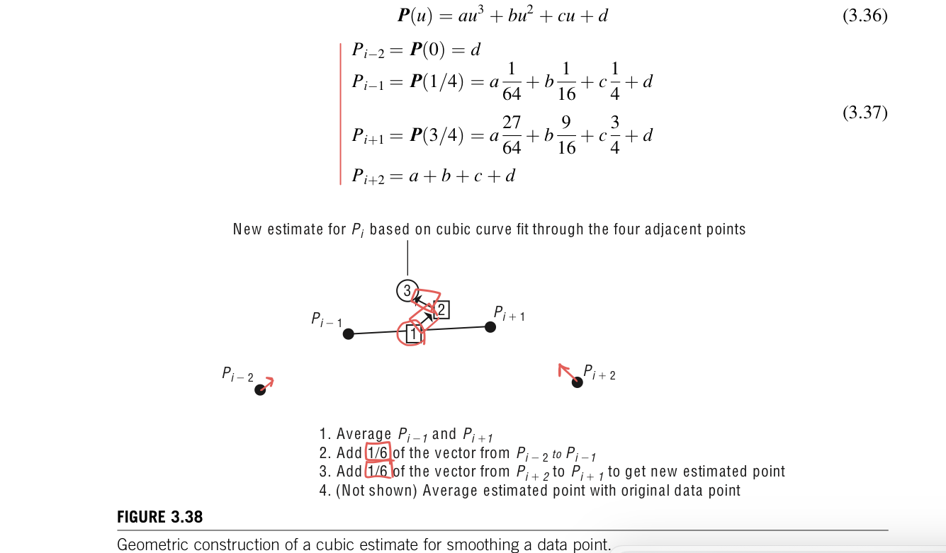
When the data to be smoothed can be viewed as a value of a function, y_i=f(x_i), the data can be smoothed by convolution. A smoothing kernel can be appliced to the data points by viewing them as a step function. Desirable attributes of a smoothing kernel include the following: it is centered around 0, symmetric, has finite support, and the area under the kernel curve equals 1. A new point is calculated by centering the kernel function at the position where the new point is to be computed. The new point is calculated by summing the area under the curve that results from multiplying the kernel function, g(u), by the corresponding segment of step function, f(x).
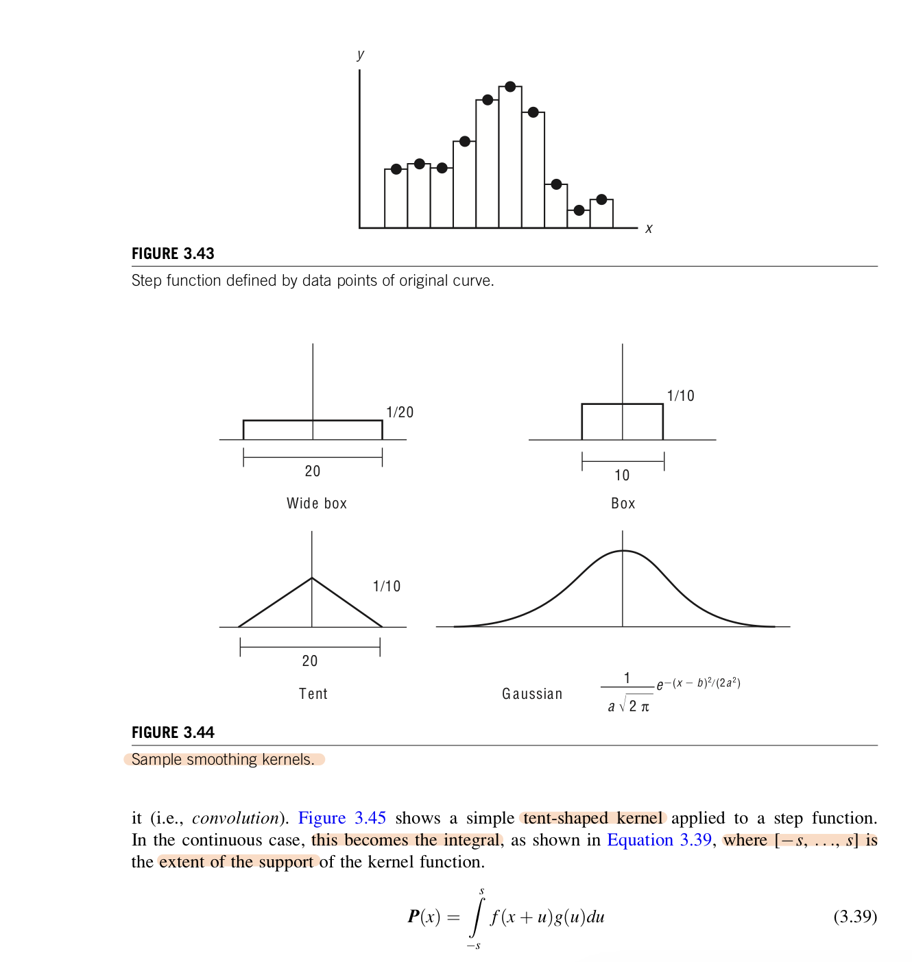
Figure 3.45 shows a simple tent-shaped kernel applied to a step function. This becomes the intergral, where [-s,...,s] is the extent of the support of the kernel function. The integral can be computed by discrete means. This can be done either with or without averaging down the number of points making up the path. At the end points, this step function can be arbitarilt extended so as to cover the kernel function when centered over the endpoints. Often the first and last points must be fixed because of animation constraints, so care must be taken in processing these.
Smoothing by B-spline approximation
if an approximation to the curve is sufficient, then points can be selected, for example, B-spline control points can be generated based on selected points. The curve can be generated using the B-spline control points, which ensure that the curve is smooth even though it no longer passes through the original points.
3.4.4 Determining a path along a surface
If one object is to move across the surface of another object, then a path across the surface must be determined.
If start and destination points are known, it can be computationally expensive to find the shorter path between the points. However, it is not often necessaary to find the absoulte shortes path. Various alternatives exist for determining suboptimal yet reasonably direct paths.
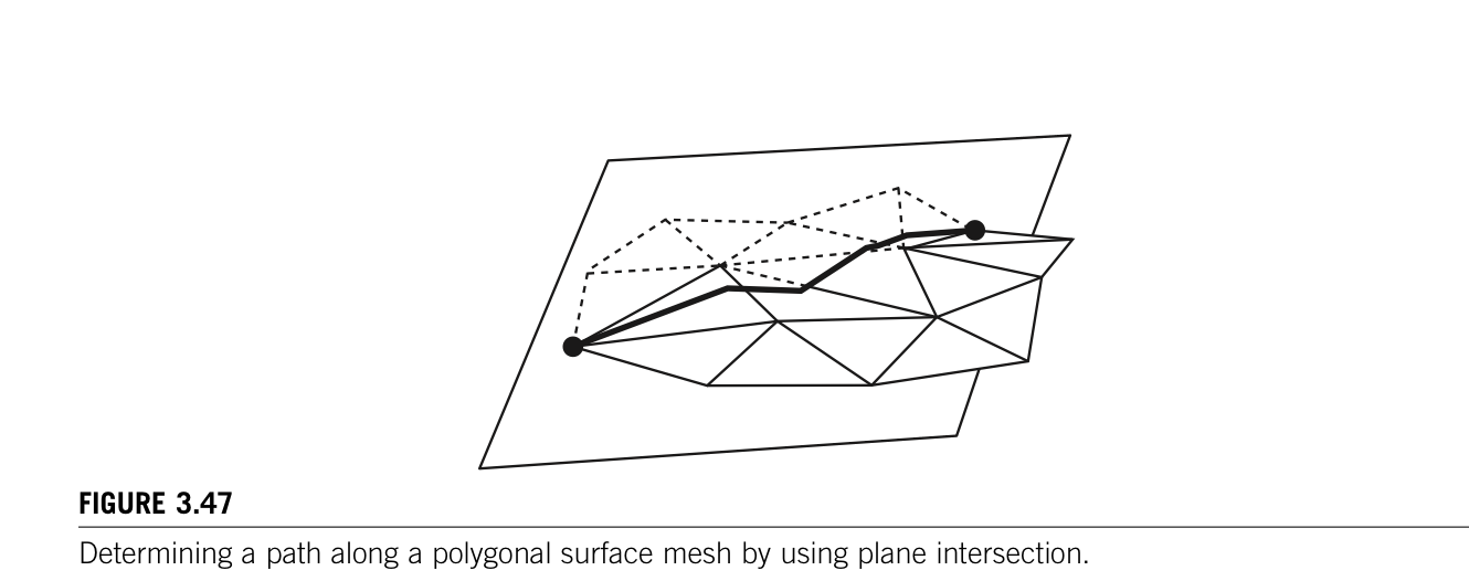
An easy way to determine a path along a polygonal surface mesh is to determine a plane that contains the two points and is generally perpendicular to the surface.
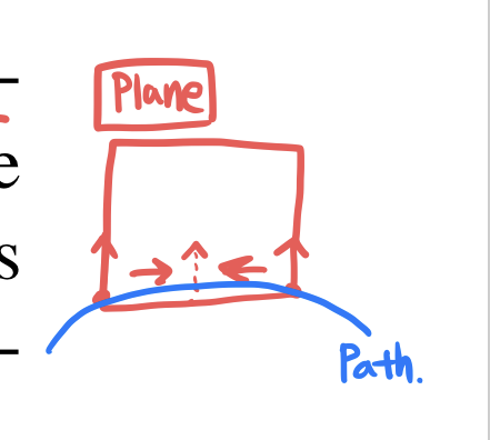
Generally perpendicular can be defined, as the plane containing two vertices and the average of the two vertex normals. The intersection of the plane with the faces will define a path between the points.
If the surface is a higher order surface and the known points are defined in the u,v coordinates, then a straight line can be defined in the parametric space and transferred to the surface. A linear interpolation of u,v does not guarantee the most direct route, but it produce a reasonaly short path.
Over a complex surface mesh, a greedy-type algorithm can be used to construct a path along a surface from a given start vertex to a given destination vertex. From each edge emanating from the current vertex, calculate the projection of the edge onto the unit vector from current to destination. Divide this distance by the length of the dege to get. The cosin of the angle between the dege and the straight line.
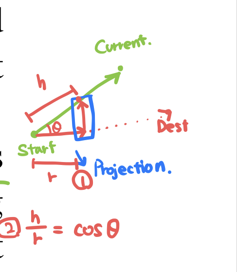
Choose this eddge to add to the path. Keep applying this until the destination edge is reached. Improvement to this approach can be made by allowing path to cut across polygons to arrive at apoints along edges. For example, using the current path point and the line from the start and end to form a aplne, intersect the plane with the plane of the current triangle. If the line of intersection falls inside of the current triangle, use segment inside of the triangle as part of the path. If the line of intersection is outside of the triangle, find the adjacent triangle and use it as the current triangle, and repeat. The start and end can be used along with some point on the surface that is judged to lie in the general direction of the path.
3.4.5 Path finding
Finding a collision-free path is a complicated task. In the simple case, a point is to be moved throuugh an otherwise stationary environment. If an obstacles are moving, but their path are known beforehand, then the problem is managebale. If the movements of the obstructions are not known, then path finding can be difficult. A further complication is when the object is not just a point but has spatial extent. If the object has a nontirivial shape and can be arbitarily rotated, then problem becomes more interesting. A few ideas for pathfinding are mentioned here.
In finding a collision-free path among static obstacles, it is often useful to break the problem into simpler subproblems by introducing via points. These are points that the path should pass through or points that the path might pass through. Finding the path is finding paths between the via points.
If the size of moving object might determine whether it can pass between obstacles, then finding a collision-free path can be a problem. However, if the object can be approximated by a sphere, then increasing the size of the obstacles changes the problem into one of finding the path of a point through the expanded environment.
Situations in which the obstacles are moving present significant challenges. A path through the static objects can be established and then movement along this path can be used to avoid moving obstalces. If the environment is not clutered with moving obstacles, then a greedy-type algorithm can be used to avoid one obstacle at a time. This type of approach assumes that the motion of the obstacles is predictable.
'ComputerGraphics' 카테고리의 다른 글
| Chapter7. Implicit line representation (0) | 2023.02.06 |
|---|---|
| Interpolation-Based Animation (0) | 2022.11.14 |
| Working with paths (0) | 2022.11.09 |
| Interpolation of orientations (0) | 2022.11.09 |
| General distance-time functions (0) | 2022.11.08 |


댓글