3.2.4 General distance-time functions
One finds that the assumption that the total distance is to be traversed during the total time presents some interesting issues. Once the total distance and total time are given, the average velocity is fixed. This average velocity must be maintained as the user modifies, for example, the shape of the velocity-time curve . This can create problem if the user is working only with the velocity-time curve. One solution is to let the absolute position of the velocity-time curve float along the velocity axis.

However, this means that if the user wants to specify certain velocities, such as starting and ending velocities, then other velocities must change in response in order to maintain total distance.
An alternative way to specify speed control is to fix the absolute velocities at key points and then change the interior shape of the curve to compensate for average velocity. However, this may result in unanticipated changes in the shape of the velocity-time-curve. Some combinations of calues may result in unnatural spikes. Consequently, undesirable accelerations may be produced.

Notice that negative velocities mean that a point traveling along the space curve backs up along the curve. Usually, this is not desirable behavior.

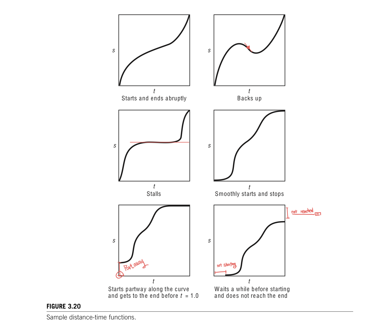
The user may also work directly with the distance-time curve. Assuming that a point starts at the beginning of the curve at t=0 and traverses the curve to arrive at the end of the curve at t=1, then the distance-time curve is constrained to start at (0,0) and end at (1,1). If the objective is to start and stop with zero velocity, then the slope at the start and end should be 0. The restriction that a point traveling along the curve may not back up any time during the traversal; the curve must be monotonically increasing(non-negative slope). If the point may not stop along the curve, then there can be no horizontal sections in the curve(no internal zero slopes).
As mentioned before, the space curve that defines the path along which the object moves is independent of the speed control curves that define the relative velocity along the path as a function of time. A single space curve could have several velocity-time curves defined along it. A single distance-time curve, such as a standard ease-in/ease-out function could be applied to several different space curves. Reusing distance-time curves is facilitated if normalized distance and time are used.
Motion control frequently requires specifying positions and speeds along the space curve at specific times(like keyframes). An example might be specifying the motion of hand. The hand accelerates toward the object and then, it slows down to almost zero speed. The motion is specified as a sequence of constraints on time,position,arc length,velocity and acceleration. Stating the problem, each point to be constrained is an n-tuple, at which all the constraints must be satisfied. Define the zero-order constraint problem take on any values necessary to meet the position constraints at the specified times. Zero-order constraned motion is illustrated in top of Figure 3.21. Notice there is continuity of position but not of speed. By extension, the first-order constraint problem requires satisfying sets of three tuples, as shown in the bottom illustration in figure 3.21.

3.2.5 Curve fitting to position-time pairs.
if the animator has specific positional constraints that must be met at specific times, then time-parameterized space curve can be determined. Position-time pairs can be specified by the animator, and the control points of the curve that produce an interpolating curve can be computed.

For example, consider the case of fitting a B-spline to values of the form (P_i, t_i)=1, ... , j. Given the form of B-spline curves shown in Equation 3.23 of degree k with n+1 defining control vertices and ecpanding in terms of the j given constraints (2<=k<=n+1<=j) results.

If there are the same number of given data points(j) as there are unknown control points(n+1), then N is square and the defining control vertices can be solved by inverting the matrix B=N^-1P
The resulting curve is smooth but can sometimes produce unwanted wiggels. Specifying fewer control points can remove these wiggles but N is no longer square. To solve the matrix equation, the use of the pseudoinverse of N is illustrated, but in practive algorithm for solving linear least-square problem should be used.

'ComputerGraphics' 카테고리의 다른 글
| Working with paths (0) | 2022.11.09 |
|---|---|
| Interpolation of orientations (0) | 2022.11.09 |
| Ease-in/Ease-out (0) | 2022.11.07 |
| Reference notice for Computer graphics category (0) | 2022.11.04 |
| Find a point that is a given distance along a curve (0) | 2022.11.04 |


댓글