3.2.3 Ease-in/Ease-out
Ease-in/out is most common ways to control motion along a curve.the standard assumption is that the motion starts and ends in a complete stop and there are no instantaneous jumps in velocity(first-order continuity). The speed control function will referred to as s=ease(t), where t is uniformly varying input parameter meant to represent time and s is the output parameter that is the distance(arc length) traveled as a function of time.
Sine interpolation
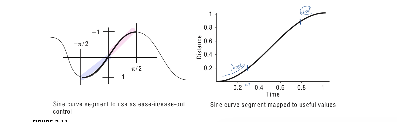
One easy way to implement ease-in/ease-out is to use section of the sine curve from -pi/2 to pi/2 as the ease(t) function. This is done by mapping the parameter values of 0 to 1 into the domain of -pi/2 to pi/2 and then mapping the corresponding range of the sin functions of -1 to 1 in the range 0 to 1.

In this function, t is the input that is to be varied uniformly from 0 to 1. The output, s also goes from 0 to 1 but does so by starting off slowly, speeding up, and then slowing down. The speed of s with respect to s is never constant over an interval, rather it is accelerating or decelerating. The derivative of this ease function is 0 at t=0 and at t=1. Zero derivative indicates a smooth acceleration from a stopped position and smooth deceleration to a stop.
Using sinusoidal pieces for acceleration and deceleration
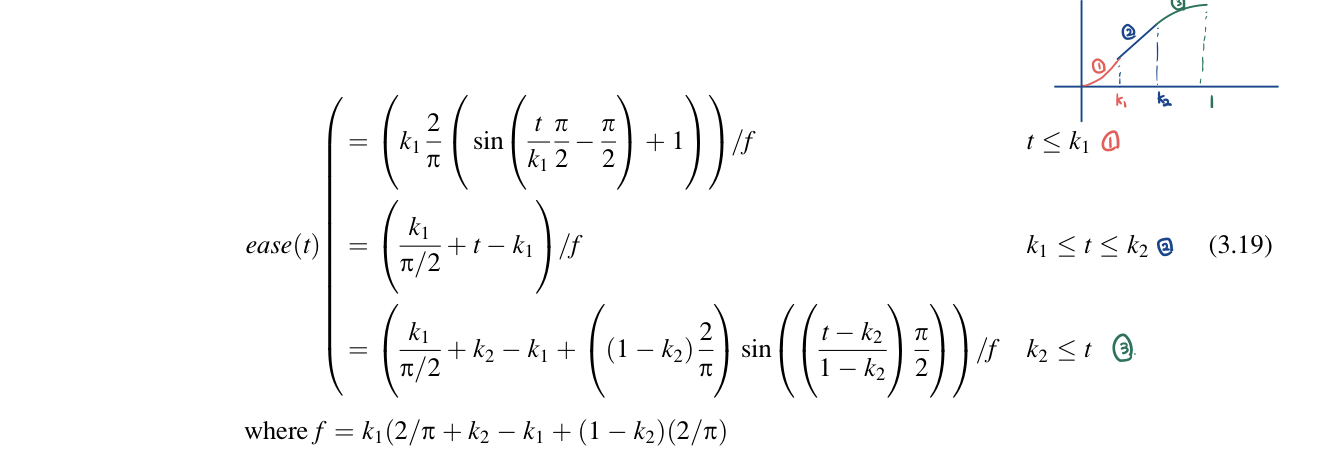
To provide an section of the distance-time function that has constant speed, pieces of the sine curve can be constructed at each end of the function with a linear intermediate segment. Care must be taken so that the tangents of the pieces line up to provide first-order continuity. Assume that the user specifies fragments of the unit interval that should be devoted to initial acceleration and final deceleration. For example, user can specifiy that acceleration ceases at 0.3 and deceleration starts at 0.75. Between times k1 and k2, constant velocity is used.
The solution is formed by piecing together a sine curve segment from -pi/2 to 0 with a straight line segment inclined at 45 degrees. The initial sine curve segment is uniformly scaled by k_1/pi/2 so that length of its domain is k_1. The sine curve segments must be uniformly scaled to preserve C^1 (first-order) continuity with the straight line segment.

Single cubic polynomial ease-in/ease-out
A single polynomial can be used to approximate the sinusoidal ease-in/ease-out control. It provides accuracy within a couple of decimal points while avoiding the transcedental function invocation. It passes through the points (0,0) and (1,1) with horizontal beginning and ending tangents of 0. Its draw back is that thare is no intermediate segment of constant speed.
Constant acceleration: parabolic ease-in/ease-out
To avoid the transcedental function, while providing for a constant speed interval between the ease-in and ease-out intervals, an alternative approach is to establish the basic form that the velocity-time curve can assume. The user can set the parameters to specify a particular velocity-time curve.
The simple case of no ease-in/out would produce a constant zero acceleration curve and a velocity curve that is a horizontal straight line. At some value v_0 over the time interval from 0 to total time t_total. The actual value of v_0 depends on the total distance covered, d_total.

In the case where normalized values of 1 are used for total distance and total time, v_0=1.
The distance-time curve is defined by the integral of the velocity-time curve and relates time and distance along the space curve through a function S(t).

To implement an ease-in/ease-out function, constant acceleration and deceleration at the beginning and end of the motion and zero acceleration during the middle of the motion are assumed. The assumption of beginning and ending with stopped position mean that velocity starts out and ends at 0. The area under the curve marked "acc" must be equal to the area above the curve marked "dec".
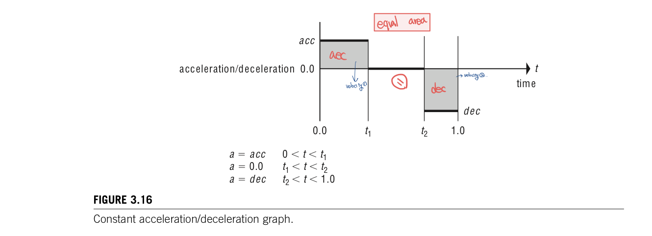
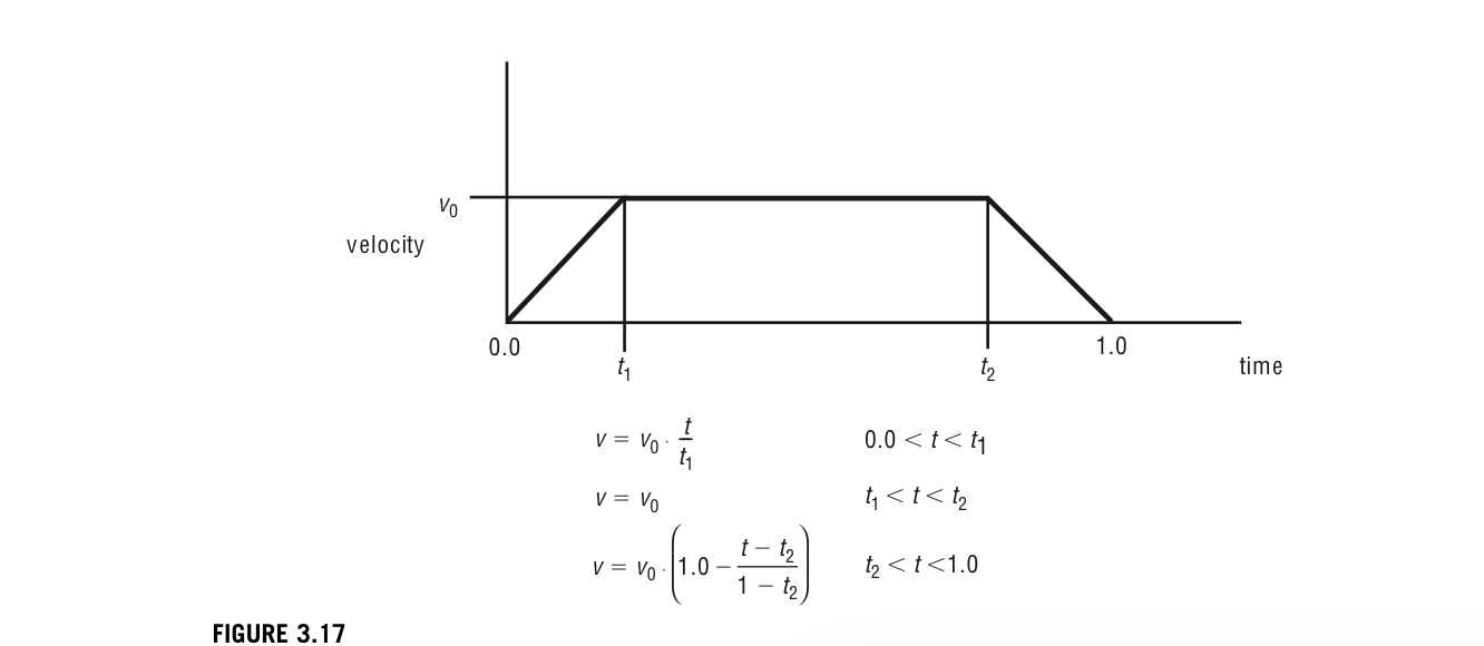
This piecewise constant acceleration function can be integrated to obtain the velocity function. The resulting velocity function has a linear ramp for accelerating, followed by a constant velocity interval, and ends with a lineaer ramp for deceleration. The integration introduces a constant into velocity. Function, but this constant is 0 under the assumption that the velocity starts out and ends at 0. The constant velocity attained during the middle interval depends on the total distance; the velocity is equal to the area velow the acc segment. In figure 3.16, in this case of normalized time and distance, the total time and distance are equal to 1.
The area under the velocity curve can be computed as in Equation 3.21
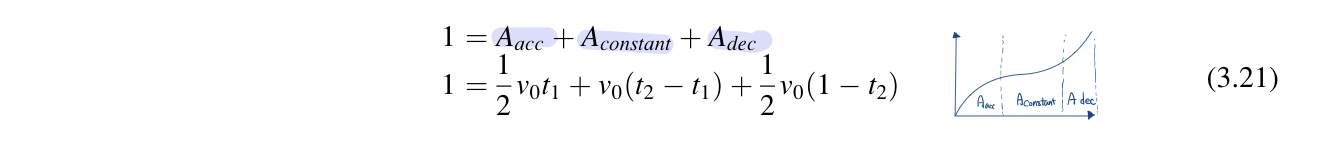
Because integration introduces arbitary constants, the acceleration-time curve does not bear any direct relation to total distance. It is more intuitive to use velocity-time curve to specify ease-in/out parameters. In this case, the user can specify three variables, t1,t2, and v0, and the system enforce the "total distance covered" constraint. For example, if the user specifies the time over which acceleration and deceleration take place, then the maximum velocity can be found.
The velocity-time function can be integrated to obtain the final distance-time function. With the assumption that the motion begins at the start of the curve, the constraint is constrained to be 0. The integration produces a parabolic ease-in segment, followed by a linear segment, followed by a parabolic ease-out segment.
The methods for ease control based on one or more sine curve segments are easy but less flexible than the acceleration-time and velocity-time function. These two functions allow the user to have more control ecause of the ability to set various parameters.
'ComputerGraphics' 카테고리의 다른 글
| Interpolation of orientations (0) | 2022.11.09 |
|---|---|
| General distance-time functions (0) | 2022.11.08 |
| Reference notice for Computer graphics category (0) | 2022.11.04 |
| Find a point that is a given distance along a curve (0) | 2022.11.04 |
| The analytic approach to computing arc length (0) | 2022.11.01 |


댓글