The analytic approach to computing arc length
The length of the curve from a point P(u_a) to P(u_b) can be found by

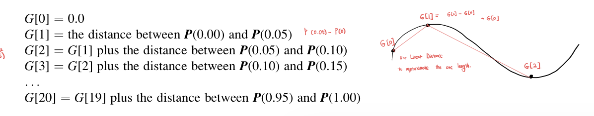
Estimating arc length by forward differencing
As mentioned, analytic techniques are not tractable for many curves. The easiest and simplest strategy for establishing the correspondence between parameter value and arc length is to sample the curve at a multitude of parametric values. Each parametric value produces a point along the curve. These sample points can be used to approximate the arc length by computing the linear distance between adjacent points. It would be computed as follows:

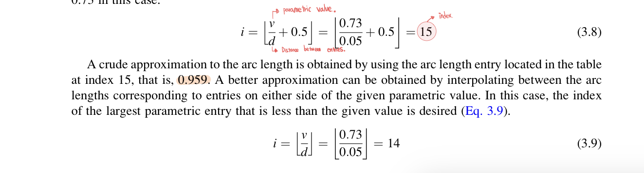
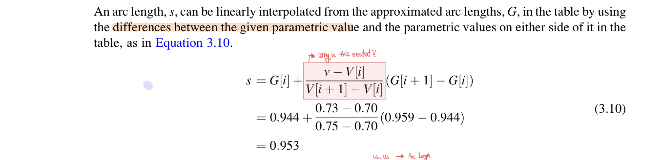
Consider the case in which the user wants to know the distance(arc length) from the beginning of the curve to the point on the curve corresponding to a parametric value of 0.73. The distance between parametric entries, d=0.05 in this case, and the given parametric value, v= 0.73.
The converse situation, that of finding the value of u igven the arc length, is dealt with in a similar manner. The table is searched for the closest arc length entry to the given arc length value. Because the arc length entries are monotonically increasing, a binary search is an effective method. As before, once the closest arc length is found, the corresponding parameter entry can be used as the approximate parametric value, or the parametric entries corresponding to arc length entries on either side of the given arc length value can be used to linearly interpolate an estimated parametric value.
For example, if the task is to estimate the location of the point on the curve that is 0.75 unit of arc length from the beginning of the curve , the table is searched for the entry whose arc length is closest to that value. In this case, the closest arc length is 0.72 and the corresponding parametric value is 0.40. The values in the table that are on either side of the given distance are used to linearly interpolate a parametric value. The value of 0.75 is three-eights of the way between 0.72 and 0.80.

the solution to the second problem(given an ar length s and a parameter value u_a, find u_b such that Length(u_a, u_b)=s) can be found by using the table to estimate the arc length. The advantages of this approach are that it is easy to implement, intuitive, and fast to compute. The downside is taht both estimate of the arc length and the interpolation of the parametric value introduce errors into the calculation. These errors can be reduced in a couple of ways. The curve can be supersampled to help reduce errors in forming the table. For example, equally spaced values of the parameter could be used to construct table consisting of entries by breaking down each interval into ten subintervals.
Better methods of interpolation can be used to reduce errors is higher-degree interpolation procedures. Of course, this slows down the computation.
Adaptive approach
To better control error, an adaptive forward differencing approach can be used that invests more computation in areas of the curve that are estimated to have large errors. The approach does this by considering a section of the curve and testing to see if the estimates for each segment's halves. If the difference is greater than can be tolerated, then the segment is split in half and each half is put on the list of segments to be tested. In addition, at each level of subdivision the tolerance is reduced by half to reflect the change in scale. If the difference is within the tolerance, then its estimated length is taken to be a good enough estimate and is used for that segment.
As before, a table is to be constructed that relates arc length to parametric value. A linked list is an appropriate structure to hold this because the number of entries is not known beforehand; after all points are generated, the linked list can then be copied to a linear list to facilitate a binary search. A sorted list of segments is maintained.
the adaptive approach begins by initializing the table with an entry for the first point of the curve <0.0,P(0)>. The procedure operates on segments until the list is empty. The first segment on the list is always the one tested next. The segment's midpoint is computed by evaluating the curve at the middle of the range of its parametric value. The curve is also evalueated at the endpoint of the segment; the position of the start the segment is already in the table and can be retrieved from there. The length of segment and the lengths of each of its halves are estimated by the linear distance between the points on the curve. The sum of estimated lengths of two halves of the segment is compared to the estimated length of segment.
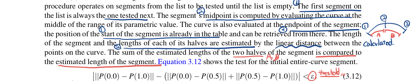
If the difference between two values is above user-specified threshold, then both halves are added to the list of segments to be tested along with their error tolerance(epsilon/2^n where n is the level of subdivision). If the values are within tolerance, then the parametric value of the midpoint is recorded in the table along with the arc length of the first point of the segment plus the distance from the first point to midpoint. Also added to the table is the last parametric value of the segment along with the arc length to the mid point plus the distance from the midpoint to the last point. When the list of segments to be tested becomes empty, a list of <parametric value, arc length> Has been generated for the entire curve.

One problem with this approach is that at a premature stage in the procedure two half segments might indicate that the subdivision can be terminated. It is usually wise to force subdivision down to a certain level and then embark(keep going) on the adaptive subdivision.
It is not possible to directly compute the index of a given parametric entry with the nonadaptive approach.

To hold the final table, a sequential search or, possibly, a binary search must be used.
Estimating the arc length integral numerically
For the cases in which efficiency of both storage and time are of concern, calculating the arc length function numerically may be desirable. Many numerical integration techniques approximate the integral of a function with the weighted sum of values of the function at various points in the interval of integration. Techniques such as Simpson's and trapezoidal integration use evenly spaced sample intervals. Gaussian quadrature uses unevenly spaced intervals to get greatest accuracy using the smallest number of function evaluations. Minimizing the number of evaluations is important for efficiency. Also, because the higher derivatives are not continuous for some piecewise curves, this should be done on a per segment basis.
Gaussian quadrature is defined over an integration interval from -1 to 1. The function is evaluated at fixed points in the interval -1 to 1, and each function evaluation is multiplied by a precalculated weight

A function, g(t), defined over interval t in [a,b] can be converted to a function h(u)=g(f(u)), defined over the interval [-1,1]. By making this substitution and the corresponding adjustments to the derivative, any range can be handled by the Gaussian integration for arbitrary limits a and b.

the weights and evaluation points for the different orders of Gaussian quadrature have been tabulated. The arc length of a cubic curve is used to define the arc length function.
Adaptive Gaussian Integration
Some space curves have derivatives that vary rapidly in some areas and slow in others. For such curves, Gaussian quadrature undersample some areas of the curve or oversample some other areas. In the former ease, unacceptable error will accumulate. In the latter case, time is wasted by unnecessary evaluations.
An adaptive approach can be used. Adaptive Gaussian integration is similar to the adaptive forward differencing. Each interval is evaluated using Gaussian quadrature. The interval is divided in half. The sum of the two halves is compared with the value calculated for the entire interval. If the difference between these two values is less than the desired accuracy, then the procedure returns the sum of two halves; otherwise the two halves are added to the list of intervals to be subdivided along with the reduced error tolerance epsilon/2^n, where epsilon is the user-supplied error tolerance and n is the level of subdivision.
The length of the entire space curve is calcualted using adaptive Gaussian quadrature. A table of the subdivision points is created. Each entry in the table is a pair (u,s) where s is the arc length at parameter value u. When calculating LENGTH(0, u), the table is searched to find the value u_i, u_i+1 such that u_i < u < u_i+1. The arc length from u_i to u is then calculated using nonadaptive Gaussian quadrature. This can be done because the space curve has been subdivided in a way that nonadaptive Gaussian quadrature will give the required accuracy over the interval from u_i to u_i+1

This solves the first problem posed above; given u_a and u_b find LENGTH(u_a,u_b). To solve the second problem of finding u, which is the given distance, s, away from the given u_a, numerical root-finding techniques must be used as described next.
'ComputerGraphics' 카테고리의 다른 글
| Reference notice for Computer graphics category (0) | 2022.11.04 |
|---|---|
| Find a point that is a given distance along a curve (0) | 2022.11.04 |
| Controlling the motion of a point along the curve (0) | 2022.10.31 |
| Interpolating Values (0) | 2022.10.31 |
| Quaternion representation (0) | 2022.10.27 |


댓글