3.1 Interpolation
The foundation of most computer animation is the interpolation of values. The interpolation of the position in space is nontrivial and requires some discussion of issues; the appropriate interpolating function, the parameterization of the function. Keep in mind that any changeable values such as an object's transparency, the camera's focal length, or the color of a light source could be subjected to interploation.
Often, an animator has a list of values associated with a given parameter at specific frames(key frames or extremes) of the animation. The question to be answered is how best to generate the values of the parameter for frames. The parameter to be interpolated may be a coordinate of the position of an object, a joint angle, the transparency or etc. The parameter of interest must be generated for all of the frames.
For example, if the animator wants the position of an object to be (-5,0,0) at frame22 and the position to be (5,0,0) at frame 67 then values fofr the position need to be generated for frames 23 to 66. Linear interpolation could be used. But what if the object needs to accelerate or decelerate at certain frame?
3.1.1 The appropriate function
In this section, the discussion covers general issues that determine how to choose the most appropriate interpolation technique: interpolation versus approximation, complexity, continuity, and global versus local control.
Interpolation versus approximation
The first discussion is whether the given values represent actual positions that the curve should pass through(interpolation) or whether they are meant merely to control the shape of the curve and do not represent the actual position that the curve will intersect(approximation). In the interpolation, the desired curve is assumed to be constrained to travel through the sample points, which is the definition of an interpolating spline. In the approximation, the animator gets a feel for how repositioning the control points influences the shape of the curve.
Commonly used interpolating functions are the Hermite formulation and the Catmull-Rom spline. The Hermite formulation requires tangent information at the endpoints, whereas Catmull-Rom uses only positions the curve should pass through. Parabolic blending requires only positional information. Functions that approximate the control information include Bezier and B-spline curves.

Complexity
It is translated into computational efficiency. The simpler the underlying equations, the faster its evaluation. In practice, polynomials are easy to compute, and piecewise cublic polynomials are the lowest degree polynomials that provide sufficient smoothness while allowing enough flexibility to satisfy other constraints such as beginning and ending positions and tangents. A polynomial whose degree is lower than cubic does not provide for a point of inflection(the way that wave goes up and down); therefore it might not fit smoothly to certain data points. Using a polynomial whose degree is higher than cubic does not provide any significant advantages and is more costly to evaluate.
Continuity
The smoothness in the curve is a primary consideration. It is determined by how many of the derivatives are continuous. Zero-order continuity refers to the continuity of values of the curve itself. If a small chane in the value of the parameter always results in a small change in the value of function(no discontinuous jump), then the curve has zero-order, or positional continuity. The first derivative of function(the instantaneous change in values of the curve) can be same, then the function has first-order, or tangential, continuity. Second-order continuity refers to continuous curvature or instantaneous change of the tangent vector. When dealing with time-distance curves, second-order continuity can be important.
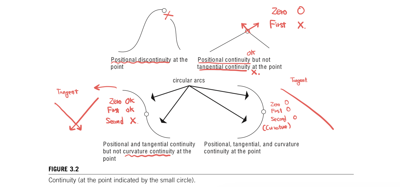
A curve interpolating or approximating more than a few points is defined piecewise; the curve is defined by a sequence of segments where each segment is defined by a single, vector-valued parametric function and share its endpoints with the adjacent segments. For many types of curve segments, the segment functions are cubic polynomials. The issue then becomes the continuity enforced at the junction between adjacent segments. Hermite, Catmull-Rom, parabolic blending, and cubic Bezier curves can all produce first-order continuity. There is a form of compound Hermite curves that produces second-order continuity. A cubic B-spline is second-order continuous everywhere.
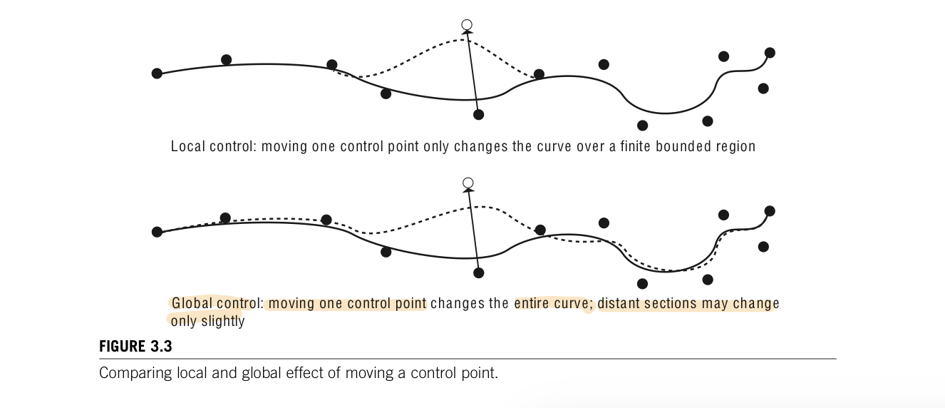
Global versus local control
When designing a curve, a user often control the shape of the curve in order to tweak just part of the curve. It is usually considered an advantage if a change in a single control point has an effect on a limited region of a curve. A formulation in which control points have a limited effect on the curve is referred to as providing local control. If repositioning one control points redefines the entire curve, then it provides only global control. Local control is viewed as being the more desirable of the two. Almost all of the composite curves provide local control: parabolic blending, Catmull-Rom, composite cubic Bezier, and cubic B-spline. Hermite curves does so at the expense of local control. Bezier and B-spline curve has less localized than their cubic forms.
There are many formulations that can be used to interpolate values. The specific formulation chosen depends on the desired continuity, whether local control is needed, the degree of computational complexity involved. The Catmull-Rom spline is used in creating a path through space because it is an interpolating spline and requires no additional information from the user other than the points that the path is to pass through. Bezier curves that are constrained to pass through given points are also used. Parabolic blending affords local control and is interpolating.
'ComputerGraphics' 카테고리의 다른 글
| The analytic approach to computing arc length (0) | 2022.11.01 |
|---|---|
| Controlling the motion of a point along the curve (0) | 2022.10.31 |
| Quaternion representation (0) | 2022.10.27 |
| Orientation representation (0) | 2022.10.26 |
| Error consideration (0) | 2022.10.24 |


댓글