Find a point that is a given distance along a curve
The solution of the equation s - LENGTH(u_a, u)=0 gives the value of u such that the point P(u) is at arc length s from the point P(u_a)

Since the arc length is a monotonically increasing function of u, the solution is unique provided that the length of dP(u)/du is not identically 0 over some interval(derivative is nonzero). Newton-Raphson iteration can be used to find the root of the equation because it converges rapidly and requires little calculation.

F is equal to s - LENGTH(u_1, U(p_n-1)) where U(p) is a function that computes the parametric value of a point on a parameterized curve. The function U() can be evaluated at p_n-1 using precomputed tables. The arc length is f' = dP/du evaluated at p_n-1(From this process we can find a point with given parametric value).
Two problems may be encountered with Newton-Rapson iteration; some of the p_n may not lie on the space curve at all, and dP/du may be 0 (we can not find the point on the curve, or it does not exist). The first problem will cause all succeeding elements p_n+1, p_n+2 to be undefined, while the latter problem will cause division by 0 or by a very small number. A zero paramteric derivative is likely to arise when two or more control points are placed in the same position.

This can easily be detected by examining the derivative of f. If it is small or 0, then binary subdivision is used instead of Newton-Raphson iteration. Binary subdivision can be used to handle undefined p_n. When finding u such that LENGTH(0, u)=s, the subdivision table is searched to find the values s_i, s_i+1 such that s_i <s <s_i+1. The solution u lies between u_i and u_i+1.
An initial approximation to the solution is made by linearly interpolating s between the endpoints of the interval and using this as the first iterate. Since each step of Newton-Raphson iteration requires evaluation of the arc length interal, eliminating the need to do adaptive Gaussian quadrature, the result is a increase in speed. The integration and root finding are completely independent of type of space curve used. The only procedure that needs to be modified is the derivative calculation subroutine.
3.2.2 Speed control
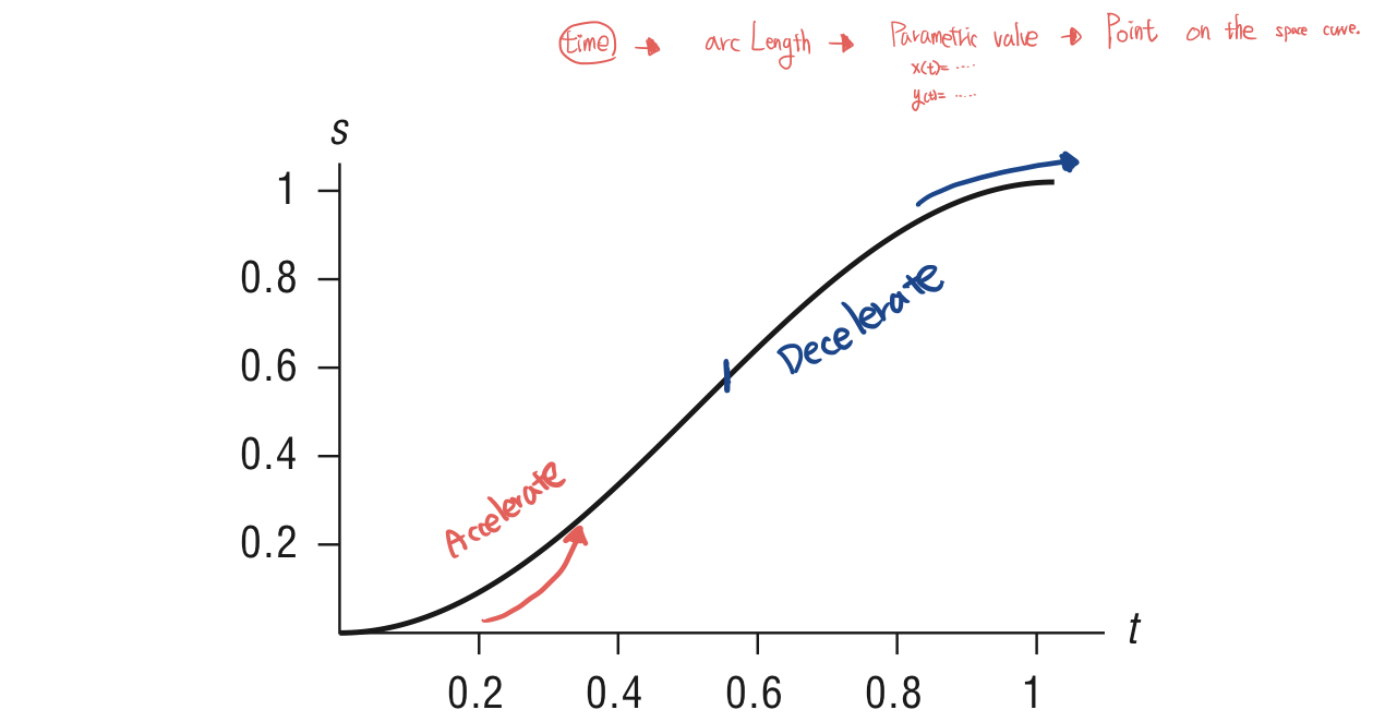
Once a space curve has been parameterized by arc length, it is possible to control the speed. Stepping along the curve at equally speed intervals of arc length will result in a constant speed traversal. The most common example of such speed control is ease-in/ease-out traversal. This type of speed control produces smooth motion as an object accelerates/decelerates.
The speed control function's input parameter is referred to as t, for time, and its output is arc length, referred to as distance or s. Constant-velocity motion along the curve can be generated by evaluating it at equally spaced values of its arc length where arc length is a linear function of t. It is much easier if, once space curve has been reparameterized by arc length, the parameterization is then normalized so that the parametric variable varies between 0 and 1. The normalized arc length parameter is just the arc length prameter divided by the total length of the curve.
Speed along the curve can be controlled by varying the arc length values; the mapping of time to arc length is independent of the form of the space curve. For example, the space curve might be linear, while the arc length parameter is controlled by a cubic function. If t is a parameter that varies in [0,1] and if the curve has been parameterized by arc length and normalized, then ease-in/out can be implemented by a function s=ease(t) so that t varies in [0,1]. Variable s is then used as the interpolation parameter.
The control of motion will be referred to as speed control. A distance-time function S(t), which, for any given time t, produces the distance traveled along the space curve(arc length). The space curve defines where to go, while the distance-time function defines when.
At a given time t, S(t) is the desired distance to have traveled along the curve at time t. The arc length of the curve segment from the beginning of the curve to the point is s=S(t). E position is used to translates along the path of the space curve at a speed indicated by S'(t). An arc length table can be used to find the corresponding parametric value u=U(s). The space curve is then evaluated at u to produce a point on the space curve, p=P(u).

There are various ways in which the distance-time function can be specified. It can be explicitly defined by giving the user graphical curve eiditing tools. It can be specified analytically, also by letting the user define the velocity-time curve, or by defining the accelration-time curve. The user can work in a combination of these spaces. In the following discussion, the assumption is that the entire arc length of the curve is to be traversed during the given total time. Two additional assumption are listed below.
1. The distance-time function should be monotonic in t, that is, the curve should be traversed without backing up along the curve.
2. The distance-time function should be continuous, that is, there should be no instantaneous jumps.
The entire curve is to be traversed in the given total time. This means that 0.0=S(0.0) and total_distance=S(total_time). The distance-time function may also be normalized so that all functions end at 1.0=S(1.0). Normalizing the function facilitates its reuse with other space curves.
'ComputerGraphics' 카테고리의 다른 글
| Ease-in/Ease-out (0) | 2022.11.07 |
|---|---|
| Reference notice for Computer graphics category (0) | 2022.11.04 |
| The analytic approach to computing arc length (0) | 2022.11.01 |
| Controlling the motion of a point along the curve (0) | 2022.10.31 |
| Interpolating Values (0) | 2022.10.31 |


댓글